Many optimization problems can be reduced to integer programming (IP) or mixed-integer programming (MIP) problems. One such problem is the Cutting Stock Problem (CSP), and in this post we focus on its 1D variant. These problems are often NP-hard (for example, the CSP is NP-hard as noted in [Wolsey, 2020]). We will compare the performance of different algorithms for solving the CSP, paying special attention to the column generation approach.
Problem Description
Imagine a paper factory that receives large sheets of paper with dimensions 1 × L (where L is a positive real number). These large sheets can only be cut along their width (each resulting piece retaining a width of 1). Therefore, for a paper piece of dimensions 1 × a, the parameter a represents its length. Assume that there is demand for paper pieces of various lengths $a_i$ (for $i = 1, \dots, n$) with corresponding demand quantities $d_i$. The objective is to minimize the number of large sheets of size L required to meet this demand.
IP Formulation
A straightforward formulation of the CSP as an integer programming problem is:
Minimize: $\quad z = \sum_{k=1}^{K} y_k$
Subject to: \(\sum_{k=1}^{K} x_{ik} \geq d_i \quad \text{for } i = 1, \dots, n\) \(\sum_{i=1}^{n} a_i x_{ik} \leq L \cdot y_k \quad \text{for } k = 1, \dots, K\) \(y_k \in \{0, 1\} \quad \text{for } k = 1, \dots, K\) \(x_{ik} \in \mathbb{Z}_+ \quad \text{for all } i = 1, \dots, n \text{ and } k = 1, \dots, K\)
Here, $y_k = 1$ indicates that the k-th large sheet is used, and $x_{ik}$ represents the number of pieces of length $a_i$ obtained from it. K is an upper bound on the number of sheets required. Note that this initial IP model can be quite inefficient due to the potentially large number of inequalities and variables.
A better formulation considers cutting patterns. A cutting pattern is a vector (of the same length as $a$) where the i-th entry tells how many pieces of size $a_i$ are produced. The pattern is valid if all entries are non-negative integers and satisfy $a \cdot k \leq L$. Let $A$ be the matrix whose columns contain all possible maximal cutting patterns (a pattern is maximal if no additional piece can be added). Suppose there are $m$ maximal patterns and let $c$ be a vector of ones with length $m$. Then, the CSP can be formulated as:
Minimize: $\quad z = c \cdot x$ Subject to: $\quad A x \geq d$ $\quad \quad \quad \quad \quad x \in \mathbb{Z}_+^m$
Algorithms and Implementation
Branch and Bound
Branch and Bound is a standard approach for solving integer programs and can be seen as a brute-force method. Below is an implementation tailored for the CSP (with some helper functions assumed to be defined elsewhere):
import numpy as np
from scipy.optimize import linprog
import math

# Assume is_integer_array, first_non_integer_index, and cp_csp are defined elsewhere
# For example:
# def is_integer_array(arr, tol=1e-6):
#     return np.all(np.abs(arr - np.round(arr)) < tol)

# def first_non_integer_index(arr, tol=1e-6):
#     for i, val in enumerate(arr):
#         if not (np.abs(val - np.round(val)) < tol):
#             return i
#     return -1 # Should not happen if called correctly

# def cp_csp(a, d, L):
#     # This function would generate the matrix A of all patterns and vector c
#     # For the purpose of this example, let's assume it returns placeholder values
#     # In a real scenario, generating ALL patterns for `A` is the hard part of this formulation.
#     # The provided B&B code actually works on the LP relaxation of the *second* formulation (with patterns).
#     # For simplicity, if 'coeffs' are passed directly to branch_and_bound,
#     # then cp_csp might not be directly called by branch_and_bound in this context.
#     # The example implies 'coeffs = cp_csp(a,d,L)' is done *before* calling branch_and_bound.
#     num_patterns = 5 # placeholder
#     num_demands = len(d)
#     c_patterns = np.ones(num_patterns)
#     A_patterns = np.random.randint(0, 5, size=(num_demands, num_patterns)) # placeholder matrix
#     return c_patterns, A_patterns, d # c, A, b (for Ax >= b, or -A, -b for linprog's A_ub x <= b_ub)


def branch_and_bound(c, A_ub, b_ub, tx, tfun, integrality_tol=1e-6): # Added A_ub, b_ub for linprog
    # Returns the best solution (lp.x) and its objective value (lp.fun)
    # Initialization: tx = [None], tfun = [float('inf')]
    """
    Expects an LP with a feasible solution.
    Similar to scipy.optimize.linprog, it minimizes the objective.
    Uses A_ub x <= b_ub form for constraints.

    tx is a list with one element (a numpy ndarray or None) and is shared.
    tfun is a list with the current best objective value.
    """
    res = linprog(c, A_ub=A_ub, b_ub=b_ub, method='highs') # Use A_ub, b_ub

    if not res.success:
        return tx[0], tfun[0]

    # Prune branch if the relaxed objective is worse than the best known.
    if res.fun >= tfun[0] - integrality_tol: # Add tolerance for comparison
        return tx[0], tfun[0]

    # If the solution is integer, update the best solution.
    non_integer_idx = -1
    for i, val in enumerate(res.x):
        if not (np.abs(val - np.round(val)) < integrality_tol):
            non_integer_idx = i
            break

    if non_integer_idx == -1: # All variables are integer
        if res.fun < tfun[0]:
            tfun[0] = res.fun
            tx[0] = res.x.copy() # Store a copy
        return tx[0], tfun[0]

    # Branch on the first non-integer variable found (non_integer_idx)
    # Branch 1: x[non_integer_idx] <= floor(res.x[non_integer_idx])
    new_row_le = np.zeros(len(c))
    new_row_le[non_integer_idx] = 1
    A_ub_le = np.vstack([A_ub, new_row_le]) if A_ub is not None else np.array([new_row_le])
    b_ub_le = np.append(b_ub, math.floor(res.x[non_integer_idx])) if b_ub is not None else np.array([math.floor(res.x[non_integer_idx])])
    branch_and_bound(c, A_ub_le, b_ub_le, tx, tfun, integrality_tol)

    # Branch 2: x[non_integer_idx] >= ceil(res.x[non_integer_idx])
    # which is -x[non_integer_idx] <= -ceil(res.x[non_integer_idx])
    new_row_ge = np.zeros(len(c))
    new_row_ge[non_integer_idx] = -1
    A_ub_ge = np.vstack([A_ub, new_row_ge]) if A_ub is not None else np.array([new_row_ge])
    b_ub_ge = np.append(b_ub, -math.ceil(res.x[non_integer_idx])) if b_ub is not None else np.array([-math.ceil(res.x[non_integer_idx])])
    branch_and_bound(c, A_ub_ge, b_ub_ge, tx, tfun, integrality_tol)

    return tx[0], tfun[0]

# Note: The csp_branch_and_bound and csp_scipy_integrality likely refer to
# the cutting pattern formulation (the second IP formulation).
# cp_csp(a, d, L) would need to generate all valid cutting patterns for matrix A.
# This is often the bottleneck for the pattern-based formulation.

# Example:
# def cp_csp(item_lengths, demands, stock_length):
#     # This is a complex function: generates all maximal cutting patterns.
#     # For a simple example, let's assume it's pre-calculated or simplified.
#     # Pattern matrix A: rows are items, columns are patterns
#     # Example: item_lengths = [3, 5], demands = [10, 7], stock_length = 12
#     # Pattern 1: four 3-unit items (4*3=12). Column: [4, 0]'
#     # Pattern 2: two 5-unit items (2*5=10). Column: [0, 2]'
#     # Pattern 3: one 5-unit, two 3-unit items (1*5+2*3=11). Column: [2, 1]'
#     # A = np.array([[4, 0, 2], [0, 2, 1]])
#     # c = np.ones(A.shape[1])
#     # b = np.array(demands)
#     # return c, A, b # c, A_patterns, demands_vector
#     pass # Placeholder

def csp_branch_and_bound(a, d, L):
    """
    Main function that uses branch and bound to solve the Cutting Stock Problem
    based on the pattern formulation.
    """
    # coeffs = cp_csp(a, d, L) # c, A_patterns, demands_vector
    # This would generate ALL patterns, which is hard. The B&B code assumes 'A_ub' and 'b_ub'
    # are for linprog's A_ub x <= b_ub. If original formulation was Ax >= d, then
    # A_ub = -A_patterns, b_ub = -demands_vector.
    # For this example, we'll skip the full cp_csp and assume coeffs are available.
    # Let's assume a simplified setup where patterns are pre-defined for B&B.
    # This part needs careful implementation of pattern generation or a different B&B approach for the first IP form.
    # The provided B&B is for the pattern formulation: min c.x s.t. Ax >= d, x integer.
    # So, for linprog: min c.x s.t. -Ax <= -d.
    # c_patterns, A_patterns, d_demands = cp_csp(a,d,L) # This is the hard part
    # A_ub_for_linprog = -A_patterns
    # b_ub_for_linprog = -d_demands
    # TX = [None]
    # TFUN = [float('inf')]
    # solution_vector, objective_value = branch_and_bound(c_patterns, A_ub_for_linprog, b_ub_for_linprog, TX, TFUN)
    # return objective_value
    print("csp_branch_and_bound requires a full implementation of cp_csp or direct pattern inputs.")
    return float('inf')


def csp_scipy_integrality(a, d, L):
    """
    Solves the Cutting Stock Problem using scipy.optimize.linprog with integrality constraints,
    based on the pattern formulation.
    """
    # coeffs = cp_csp(a, d, L) # c, A_patterns, demands_vector
    # c_patterns, A_patterns, d_demands = coeffs
    # res = linprog(c_patterns, A_ub=-A_patterns, b_ub=-d_demands, integrality=1, method='highs')
    # if res.success:
    #     return res.fun
    # else:
    #     return float('inf')
    print("csp_scipy_integrality requires a full implementation of cp_csp or direct pattern inputs.")
    return float('inf')
Note: Functions such as is_integer_array, first_non_integer_index, and cp_csp are assumed to be defined elsewhere. The B&B implementation seems geared towards the pattern-based formulation, where cp_csp would generate all patterns, which is itself a hard problem. For a practical B&B on the first IP formulation, the structure would be different. The scipy version with integrality=1 is more straightforward if you can formulate the problem for it.
Column Generation
Column Generation was originally developed for the CSP and later applied to other problems. The idea is to start with a limited set of basic columns—each corresponding to a cutting pattern that uses the maximum number of pieces of one type—and then iteratively add a new column that improves the objective value. To decide which column to add, one solves a knapsack problem based on the dual values from the LP relaxation. Although this method provides a good approximation, it does not always guarantee the optimal integer solution. For an exact solution, one could apply branch-and-price methods.
import numpy as np
from scipy.optimize import linprog
# from knapsack import knapsack # Assuming knapsack.py is in the same directory or installable

# Dummy knapsack function for completeness if not available
def knapsack_dummy(l, v, L_capacity):
    # This is a placeholder. A real knapsack solver is needed.
    # For CSP pricing, we want to maximize sum(v_i * x_i) s.t. sum(l_i * x_i) <= L_capacity
    # where v_i are duals and l_i are item_lengths.
    # Returns (max_value, solution_vector_x_i)
    n_items = len(l)
    # Simple greedy approach (not optimal for 0-1 or integer knapsack)
    # This needs to be a proper integer knapsack solver.
    print("Warning: Using dummy knapsack solver. Results will be incorrect for column generation.")
    best_val = 0
    best_sol = np.zeros(n_items, dtype=int)
    # Example: if any v_i > 0 and l_i <= L_capacity, pick one.
    # This is highly simplified and incorrect for the actual problem.
    for i in range(n_items):
        if v[i] > 0 and l[i] <= L_capacity: # Example logic for a single item
            num_can_fit = L_capacity // l[i]
            if num_can_fit > 0 :
                 # This is not how the knapsack for pricing problem works generally
                 # It needs to find the best combination.
                # For this dummy, just take one if it improves.
                if v[i] * 1 > best_val: # Simplistic
                    best_val = v[i] * 1
                    best_sol_temp = np.zeros(n_items, dtype=int)
                    best_sol_temp[i] = 1
                    best_sol = best_sol_temp
    return best_val, best_sol


def csp_generating_columns(a, d, L, knapsack_solver=knapsack_dummy): # Allow passing knapsack solver
    """
    Solves the Cutting Stock Problem using the column generation method.
    Begins with basic columns where each column uses the maximum
    number of pieces of a particular length.
    Iteratively adds columns based on solving a knapsack problem until no
    column with a negative reduced cost is found.
    """
    n = len(a)
    # Initialize basic columns (identity patterns, how many of one item fit)
    initial_columns_list = []
    for i in range(n):
        new_col = np.zeros(n, dtype=int)
        if a[i] > L:
            # If an item is larger than the stock, it can't be cut.
            # This implies an infeasible demand if d[i] > 0.
            # For column generation, we'd typically assume demands are feasible.
            # If a[i] <= L, then at least one can be cut.
            if d[i] > 0 : # Only add if demanded and possible
                 print(f"Warning: Item {i} with length {a[i]} may be too large for stock L={L} if not handled.")
            # Fallback: if an item is too large, its column might be all zeros or not included if it can't be cut.
            # Or, we can ensure a[i] <= L for all items initially.
            # For now, let's assume a[i] <= L.
            new_col[i] = L // a[i]
        else:
            new_col[i] = L // a[i]

        if new_col[i] == 0 and d[i] > 0 and a[i] <=L : # Should not happen if a[i] <= L and L > 0
             print(f"Error: Item {i} of length {a[i]} cannot be cut from stock L={L}, but demand exists.")
             # return float('inf'), float('inf'), None, None # Indicate error

        initial_columns_list.append(new_col)

    A_patterns = np.column_stack(initial_columns_list)

    # Objective coefficients (cost of using each pattern is 1)
    c_coeffs = np.ones(A_patterns.shape[1])

    iteration = 0
    max_iterations = 100 # Safety break

    while iteration < max_iterations:
        iteration += 1
        # Solve the Restricted Master Problem (RMP)
        # min c.x s.t. A_patterns.x >= d, x >= 0
        # For linprog: min c.x s.t. -A_patterns.x <= -d
        # bounds = [(0, None) for _ in range(A_patterns.shape[1])] # x_j >= 0

        # Check for empty A_patterns (e.g. if all items are larger than L)
        if A_patterns.shape[1] == 0:
            print("No valid initial patterns. Problem might be infeasible or items too large.")
            # This means demand cannot be met. If d is all zero, obj is 0.
            # If d has positive values, this is an issue.
            is_demand_zero = np.all(np.array(d) <= 1e-9)
            if is_demand_zero:
                return 0, 0, np.array([]), np.array([[]])
            else:
                print("Demand exists but no patterns generated. Infeasible.")
                return float('inf'), float('inf'), None, None


        # Solve the RMP
        # primal_res = linprog(c=c_coeffs, A_ub=-A_patterns, b_ub=-np.array(d), bounds=bounds, method='highs')
        # scipy linprog's default bounds are (0, None) already
        primal_res = linprog(c=c_coeffs, A_ub=-A_patterns, b_ub=-np.array(d), method='highs')

        if not primal_res.success:
            print(f"RMP solve failed at iteration {iteration}. Status: {primal_res.message}")
            # This could happen if -d is not feasible with -A_patterns (e.g. d is too high for current patterns)
            # Try to add more patterns or check problem formulation
            # For now, let's break and return current best if any, or error.
            # This usually indicates an issue with initial patterns or extreme demands.
            # Consider adding slack variables to RMP to ensure feasibility if this is common.
            if 'fun' in primal_res: # if it partially solved
                 current_fun_val = primal_res.fun
                 current_x = primal_res.x if 'x' in primal_res else np.zeros(len(c_coeffs))
                 return current_fun_val, np.sum(np.ceil(current_x) if current_x is not None else 0), current_x, A_patterns
            else: # Total failure
                 return float('inf'), float('inf'), None, None


        # Get dual variables for the demand constraints (A_patterns.x >= d)
        # For A_ub x <= b_ub, marginals are non-positive.
        # We want duals for Ax >= d. If pi are duals for Ax >=d, then for -Ax <= -d, duals are -pi.
        # So, if linprog gives 'duals_ub', these correspond to -Ax <= -d.
        # Duals for Ax >= d would be -duals_ub.
        # SciPy's .marginals for ineqlin are for A_ub @ x <= b_ub
        # These duals (lambda) should be non-positive.
        # The pricing problem wants to maximize sum(lambda_i * pattern_col_i) - cost_of_pattern
        # which is sum(-duals_from_scipy_i * pattern_col_i) - 1
        # Or, minimize 1 - sum(duals_for_Ax_ge_d_i * pattern_col_i)

        duals_for_Ax_ge_d = -primal_res.ineqlin.marginals # These should be >= 0

        # Solve the subproblem (Knapsack problem)
        # We want to find a new pattern (column k_new) that maximizes duals^T * k_new
        # The values for knapsack are the dual variables. Weights are item lengths 'a'. Capacity is 'L'.
        knapsack_value, new_pattern = knapsack_solver(l=a, v=duals_for_Ax_ge_d, L_capacity=L)

        # Calculate reduced cost: 1 - (duals^T * new_pattern)
        reduced_cost = 1 - knapsack_value

        if reduced_cost >= -1e-6: # No column with negative reduced cost found (allow small tolerance)
            break # Optimality reached for LP relaxation

        # Add the new pattern (column) to A_patterns
        A_patterns = np.column_stack((A_patterns, new_pattern))
        c_coeffs = np.append(c_coeffs, 1) # Cost of new pattern is 1

        # Optional: Remove non-basic columns (columns with x_j near zero) to keep RMP small
        # This is heuristic and can sometimes remove columns that might become basic later.
        # if primal_res.x is not None:
        #     active_indices = primal_res.x > 1e-8
        #     if np.any(active_indices): # Ensure not all are removed
        #         A_patterns = A_patterns[:, active_indices]
        #         c_coeffs = c_coeffs[active_indices]
        #     else: # if all are zero, something is odd, maybe keep all
        #         pass


    # LP relaxation optimal value
    lower_bound_lp = primal_res.fun
    x_lp_solution = primal_res.x

    # Get an integer solution (e.g., by rounding up, though not guaranteed optimal for IP)
    # For CSP, simply rounding up the number of times each pattern is used is a common heuristic.
    if x_lp_solution is not None:
        x_integer_heuristic = np.ceil(x_lp_solution)
        achieved_obj_heuristic = np.sum(x_integer_heuristic)
    else: # Should not happen if loop broke due to optimality
        x_integer_heuristic = np.array([])
        achieved_obj_heuristic = float('inf') if not np.all(np.array(d) <= 1e-9) else 0


    return lower_bound_lp, achieved_obj_heuristic, x_integer_heuristic, A_patterns
The figures below illustrate the performance of the implemented algorithms on various inputs:
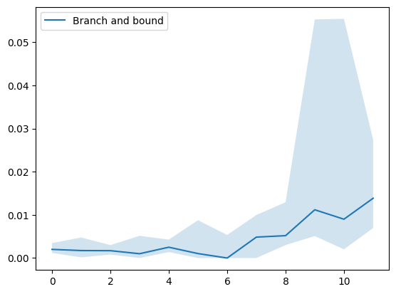
Figure 1: Performance of the branch and bound algorithm using generated inputs.

Figure 2: Performance of scipy.optimize.linprog with integrality=1.

Figure 3: Performance of the column generation algorithm.
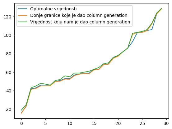
Figure 4: Approximation quality of the column generation method compared to the optimal solution. Blue represents the optimal solution, orange represents the lower bound given by the column generation method, and green represents the solution given by the column generation method.
Discussion
Although we have not delved deeply into the original IP formulation, it can be useful in certain scenarios (for instance, when large sheets vary in size). For small instances, branch and bound may be more effective. In contrast, column generation scales better for large problems since a one-unit difference in the solution is often less significant. It is important to note that the column generation algorithm is approximate and, in rare cases, may loop indefinitely if a newly added column is not used. Our implementation safeguards against that by terminating when such a scenario is detected.
Additional Materials
The complete code and implementation details are available on GitHub. There you can also find examples of how the functions are used and performance comparisons of the algorithms.
References
-
Wolsey, L. A. (2020). Integer Programming.
-
Vance, P. (1998). Branch and Price: A Method for Solving Cutting Stock Problems.
Appendix: Knapsack Problem
In the column generation method for CSP, a knapsack problem must be solved to determine the optimal column to add. Below is a dynamic programming implementation of the knapsack algorithm that runs in 𝑂 ( 𝐿 ⋅ 𝑛 ) O(L⋅n) , where L is the knapsack capacity and n is the number of item types.
import numpy as np
from copy import copy # 'copy' might not be needed if DP[i-l[j]][1] is a numpy array, as slicing creates a view/copy depending on context.
                      # For lists of lists, 'copy' or 'deepcopy' is important.
                      # If DP[i-l[j]][1] is a numpy array, direct assignment then modification is fine.

def knapsack(l, v, L_capacity): # Renamed L to L_capacity to avoid conflict with item_lengths 'l'
    """
    Solves the integer knapsack problem (unbounded knapsack variant for CSP pricing).
    l: list of item sizes (weights)
    v: list of item values (duals)
    L_capacity: knapsack capacity (stock length)
    Returns a tuple: (objective value, solution vector - how many of each item type)
    """
    n = len(l)
    # DP[i] = [max value, solution vector for that max value] for capacity i
    # Initialize solution vectors as numpy arrays for easier manipulation
    DP = [[0, np.zeros(n, dtype=int)] for _ in range(L_capacity + 1)]

    for i in range(1, L_capacity + 1): # Iterate through capacities from 1 to L
        for j in range(n): # Iterate through item types
            if l[j] <= i: # If item j can fit in current capacity i
                # Value if we include one more of item j
                # This is for unbounded knapsack: DP[i-l[j]][0] is optimal value for capacity i-l[j]
                # to which we add v[j] and one more of item j.
                current_value_if_item_j_added = DP[i - l[j]][0] + v[j]

                if current_value_if_item_j_added > DP[i][0]:
                    DP[i][0] = current_value_if_item_j_added
                    DP[i][1] = DP[i - l[j]][1].copy() # Take the solution for capacity i-l[j]
                    DP[i][1][j] += 1 # And add one more of item j
            # If item j cannot fit, or including it doesn't improve,
            # DP[i] might be better off taking the solution from DP[i-1] (if items are ordered by size)
            # or by considering other items. The outer loop for 'i' and inner for 'j' handles this.
            # However, to ensure DP[i] considers not taking item j at all but being optimal from previous items for capacity i:
            # This DP structure inherently builds up. DP[i] will be optimal using items 0..j-1 for capacity i
            # *before* considering item j for capacity i.
            # The formulation above is standard for unbounded knapsack.

    return DP[L_capacity] # Returns [max_total_value, counts_of_each_item_type]